
Objective:
In this lab, I explored how scale affects the observed relations amongst crime occurrences and census variables, and explore some of ArcGIS’s data manipulation and presentation techniques. In particular, I used a simple regression analysis to model the relation between residential break and enter crimes (B & E’s) and the total number of households and the median total household income.

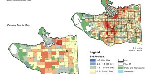
Two maps above present similar overall crime distribution. However, an CT includes several DAs, so the DA map has higher resolution and shows more details. Also, given a smaller R square value and a smaller moran’s I value, the DA map are more discrete and less clustered than the CT map, and the number of residential B & E’s is less correlated with the median household income and the total number of households in DA.

The two maps above show the results of a grouping analysis between different criminal activities and the median household income in Vancouver. The occurrence of criminal activities varies in different levels of median household income. Each color scheme represents a similar pattern of crime and its associated income level. The results shown in census tracts map gives more general spatial distribution patterns of crimes and median household income. While the map of dissemination areas provides more specific and detailed results in each community.
The map results show that areas of the city with higher median incomes are not necessary to have a lower/higher level of criminal activities. Each income level is more correlated with specific type of crime; for example, in low income neighborhoods, there is a higher chance of auto crime while in high income area, residents tend to experience more B & E crime.