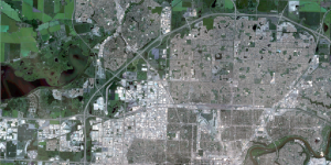
The City of Edmonton aims to determine the location and dominance of land cover types in the northern half of Edmonton, AB. The City staff have requested that Landsat 8 OLI data from August 3rd, 2017 be used in the analysis. As a result, the six land cover types, including water, road, residential, industrial, grassland/forest, and agricultural, were classified, and their corresponding locations were relatively clearly determined. In particular, the industrial and agricultural classes were clearly identified, while the road and water classes were misclassified. The classified and calculated results showed that the dominant land cover type could be either grassland/forest or residential.
Analysis
Unsupervised classification

Figure 1. Six land cover types classified by ISO (unsupervised) classification

Figure 2. ISO (unsupervised) classification filtered by FOUR HALF
At first, I used the dendrogram to conduct the unsupervised classification, but when it comes to level 4, the road feature seemed to be discontinuous and began to merge with the grassland on the two sides of the road. In order to keep the road feature, instead of continuing to use the dendrogram, I manually performed the rest of the classification after level 3 by comparing to the clipped true color image using the swipe tool. As a result, based on the land cover types identified from the true color image at the beginning, I classified 40 classes into 6 classes which are water, road, residential, industrial, grassland/forest, and agricultural (see fig 1.). After that, in order to reduce the noise and remove the single, misclassified cells, I created a filtered image using the majority filter (fig 2.), and the combinations of options in the majority filter I used are FOUR HALF. With the number of neighbors set to 4, contiguous is defined as sharing a corner. As the Replacement threshold is set to HALF and two values occur as equal portions, no replacement will occur if the value of the processing cell is the same as one of the halves.
From both fig 1. and 2., we can see that the residential and industrial classes were relatively clearly distinct classes since the locations of these two classes match their locations in the true color image, and their corresponding areas look similar in both images. Whereas, other classes seem less distinct. Compared to the true color image, the main roads, such as highways, were better classified than other roads such as the roads within residential areas. It is obvious to see that the area of water class seems to be overestimated in the ISO classification image, while the areas of grassland/forest and agricultural classes could be underestimated.
For the calculation of hectares, since the resolution of the image is 30m, I used the pixel counts for each class (i.e. 67945 for water) time the area of each pixel (i.e. 30m * 30m = 900m^2) to get the total area for each class. Both table 2. and 3. demonstrate the dominance land cover type is grassland/forest, about 28% of the total area.
Supervised classification

Figure 3. Six land cover types classified by MLC (supervised classification)

Figure 4. MLC image filtered by FOUR HALF

Figure 5. Image of output confidence raster for MLC results
The image above (Fig 5.) illustrates the output confidence raster for the MLC results, which can help us see how well the classification works. The red areas represent low confidence in the MLC results. For example, we can see from the image that the MLC works poorly on the water area at the bottom right corner, as well as the vegetation areas on the top and within the residential areas. On the contrary, the areas in green indicate high confidence in MLC results. For instance, the agricultural area on the top right corner, the water area on the middle left side, and most of the buildup areas. In general, from the histogram, we can see that a large portion of the areas is in mid confidence range.
For the supervised classification, I created 5 or 6 training sites per class and assigned hundreds to thousands of pixels to each class. However, as I mentioned above, the separability shown in histograms and scatterplots seems a little bit poor, and only industrial class shows the best separation. After that, I run the Maximum Likelihood Classification (MLC) supervised classification and produced an Output Confidence Raster from the MLC results (see fig 3. & 5.). The majority filter with the combination of Four Half was also applied to the MLC results to enhance the image (fig 12.).
From figure 3. and 4., we can see that the residential and agricultural classes were relatively clearly distinct classes since the locations of these two classes match their locations in the true color image, and their corresponding areas look similar in both images. Whereas, other classes seem less successful. Compared to the true color image, the main roads, such as highways, were better classified than other roads such as the roads within residential areas. It is obvious to see that the water area on the bottom right corner was misclassified into industrial class. Besides, the main roads such as highways are much wider than their original width, which indicates that some grassland and industrial areas might be misclassified into road class. Therefore, the area of road class still seems to be overestimated in the MLC results, while the areas of grassland/forest and industrial classes could be underestimated.
Conclusion
Although the results are not perfect and accurate enough, the two classification methods established an acceptable level of agreement, and the overall classification process visually illustrated the distribution and location of selected six features. Also, the dominance (area in hectares) of land use type was determined for each classification method, which is grassland/forest (15287.85 hectares) by the unsupervised classification, while it is residential area (17071.02 hectares) by supervised classification. In particular, the industrial and agricultural classes were clearly identified, while the road and water classes were clearly misclassified.
The classification routine I would recommend for land cover identification would still be performing the unsupervised classification prior to the supervised classification. By doing the unsupervised classification, we can acquire relatively accurate results based on the software analysis of an image without the user providing sample classes. The computer uses techniques to determine which pixels are related and groups them into classes. Unsupervised classification is fairly quick and easy to run. There is no extensive prior knowledge of area required. The classes are created purely based on spectral information; therefore, they are not as subjective as manual visual interpretation. After that, we can do the accuracy assessment and improve the classification by doing the supervised classification which is based on the idea that a user can select sample pixels in an image that are representative of specific classes and then direct the image processing software to use these training sites as references for the classification of all other pixels in the image.
For the future classification project, I would consider merging the subclasses since the clusters in training samples are sort of overlapped and poorly separated, and other new classes could be created such as swamp. Also, more training sites (i.e. 7 or 8 per class) would be created to increase the accuracy level for the MLC. Furthermore, I would rely less on the dendrogram and start to manually classify at level 1 or 2. In addition, the impacts of cloud or cloud shadows would be considered in the future.